Split Nodes
Split nodes are used to split the previous incoming node into multiple outgoing nodes (or outputs), as opposed to flowing into a single output. All nodes, except for multi-select Tables and Target nodes, can have multiple ‘split nodes’ connected to them. This splitting mechanism enables the creation of complex data flow processes. For instance, you could connect multiple filter nodes to a single table to produce multiple filtered outputs. Or you could connect several scripting nodes to a single table.
Which Nodes Can be Split?
All nodes, except for Tables and Target nodes, can be split:
- Data Source nodes: commonly split by connecting multiple Select nodes. Often this is several tables from the datasource, but it could also be multiple Query or Top or Bottom n nodes.
- Table nodes: each table node can have multiple column operations, preparations, machine learning, and scripting nodes connected.
- Top n and Bottom n nodes: like Table nodes, each Top or Bottom n node can have many outputs.
- Join nodes: merge and union nodes can be split by connecting multiple outputs.
- Column Operation nodes: can be split by connecting multiple outputs.
- Preparation nodes: can be split by connecting multiple outputs.
- Machine Learning nodes: can be split by connecting multiple outputs.
- Scripting nodes: can be split by connecting multiple outputs.
How to Split Nodes
Splitting is achieved simply by connecting the required function directly to the previous node. The result is that the node will have multiple outputs, rather than just one.
In the image below, the Filter node was split by having both a Summarize and Target node connected directly to it:

To achieve this, the source table must be split to three outputs: each of the 2 Date Range nodes and the Target node.
Once each date range is extracted, their rows are combined using the Union node, before applying Time Intelligence to generate a range of date/ time groupings.

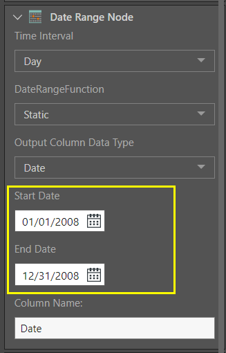
Let's take a look at this in more detail. The first Date Range node is used to extract a list of all dates from 2008:
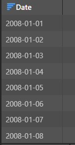
This produces a table consisting of a single column:
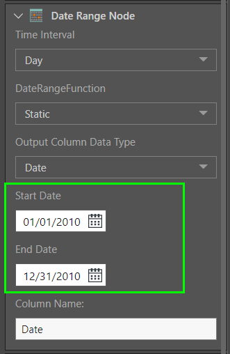
The second Date Range node is used to extract a list of all dates from 2010:
This also produces a table made up of one column:
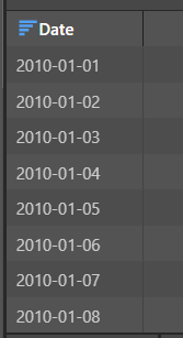
Before applying Time Intelligence, we want to combine both of the date range lists using the Union node (orange highlight below). This produces a new table made up of one column containing both date ranges:
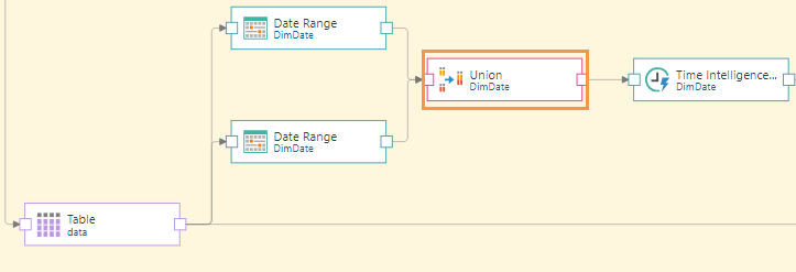
Next, the Time Intelligence node is connected to the Union node (green highlight below), and finally, the target is connected to the flow (blue highlight). It must be connected directly to the source table containing the original dateKey column (orange highlight), otherwise this table will not be included in the data model.

In this example, we want to filter the table above the average income, using the Filter node. To do this, we need the data flow to find the average income, which requires us to connect the Summarize node. One option would be to connect the Summarize node to the table and configure it to return the average income, and then connect the Filter node to the Summarize node.
However, this would require the data modeler to manually input the average from the Summarize node into the Filter node (red highlight below). Because we expect the average to change, we want this process to be automated. This requires the use of a variable.

So the solution is to create a variable 'AveIncome', and connect the Filter node directly to the Table, filtering above the variable. Then split the Filter node by connecting both the Summarize and Target nodes to it. The summarize node us used to find the average income, and the variable is fed into it.

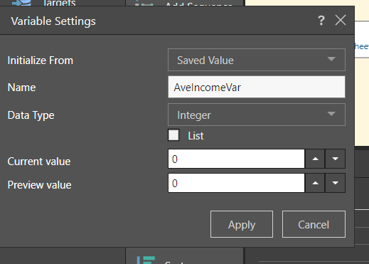
Let's look at these steps in more detail. First, the variable is created and assigned to the Integer data type:
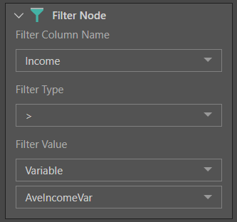
Next, the Filter node is connected to the table containing the Income column. Income is set as the filter column, the filter type is > and the filter value is the AveIncome variable.
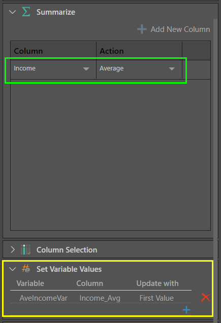
At this point, we need to tell the variable what the average income actually is. To do this, the Summarize node is connected to the Filter node, and a new Average Income column is created (green highlight below). The variable is fed into the Summarize node (yellow highlight), so that the Average Income value will be loaded into the variable.
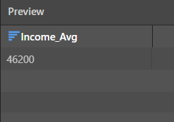
When the Summarize node is previewed, we see the average income:
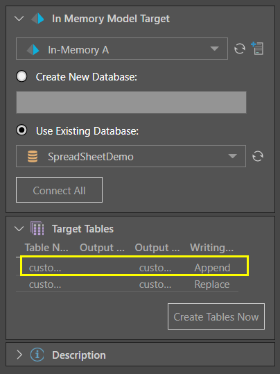
Split the Filter node by also connecting it to the Target node. Connect the Summarize node to the target as well. Change the writing type for the table generate by the Filter node to Append to ensure incremental loading.
At this point, the data flow looks like this:

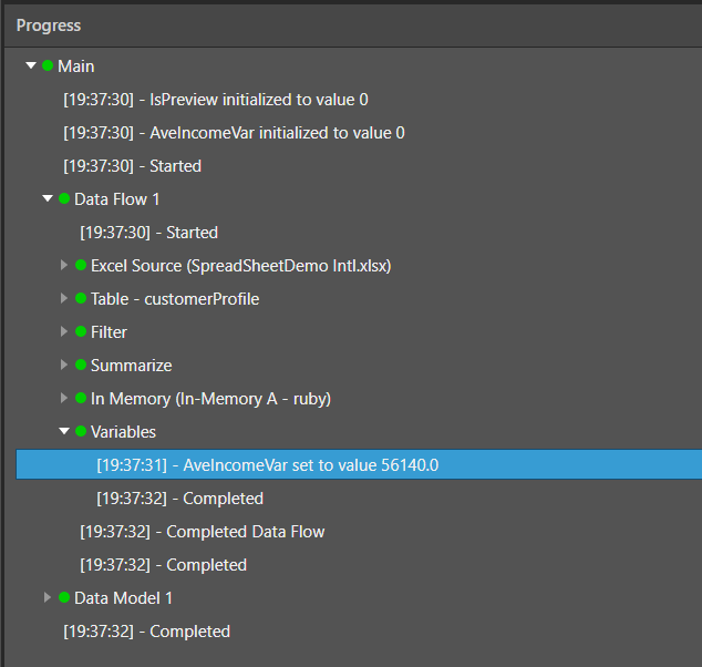
After processing the data flow, the variable output is seen in the Progress panel. It shows that the variable's value was set to the first value above the average, as specified from the summarize node.
